Union-Find algorithms in Ruby
It’s always interesting to learn something new, especially if it’s fundamental knowledge.
Recently I have found a very interesting course about algorithms. Lectures are meaningful and practical. I recommend them to everyone who wants to understand basic algorithms.
All algorithms are implemented in Java, but I decided to write them in Ruby too. In my view, it doesn’t matter what language you choose in this case. The main goal is to better understand these algorithms.
So, in this post, I want to tell you about Union-Find (UF) algorithms.
Dynamic connectivity
Firstly, we should understand the reason of this type of algorithm. Just have a look at the picture:
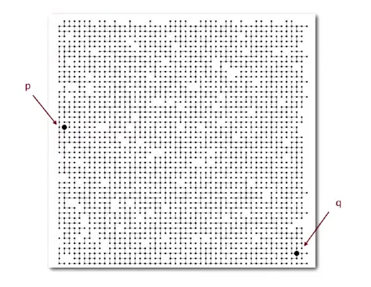
As you can see, there are 2 points: p and q. Question: is there a path between p and q?
Not so easy to answer, right? 🙂
This type of problem is called the connectivity problem. Wikipedia says:
In computing and graph theory, a dynamic connectivity structure is a data structure that dynamically maintains information about the connected components of a graph.
So, dynamic connectivity is a data structure, which can be used for describing a graph. But, what does it mean? How can we use it for answering the question?
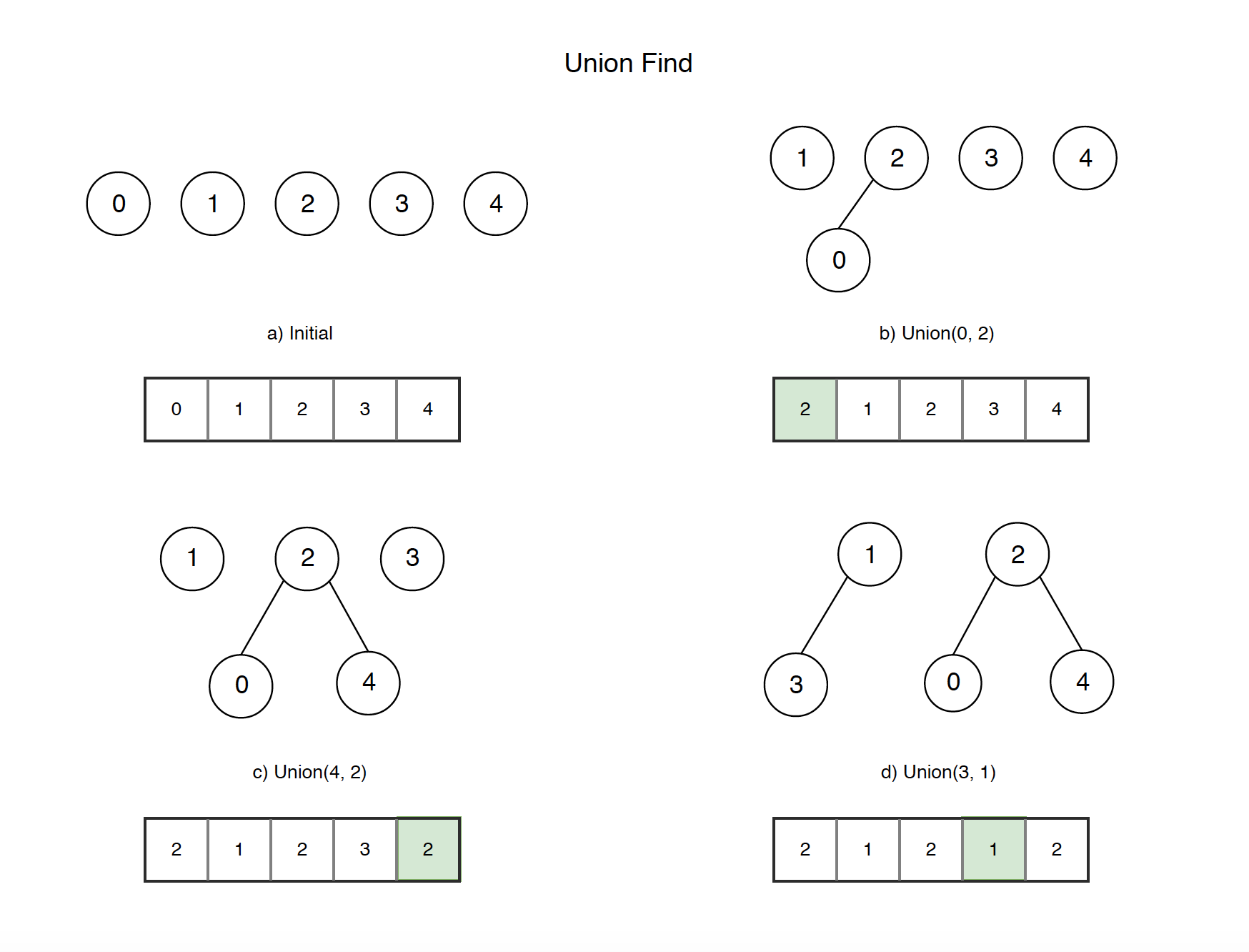
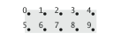
It means, we can describe the way from p to q through the graph of elements. Each element is a point, which can be connected with another one. For example, let’s say we have 10 objects and they are separated initially (they are independent components):
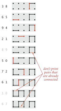
We can connect and check if some of them are already connected. The connection action is called union. TheFind is an operation that checks if two objects are in the same component. So, we can union 4 with 3:

Here are more connectivity examples:
Now, we know what is the dynamic connectivity, but how can we implement it? There are some algorithms to do Union-Find operations.
Quick-Find
The Quick Find is the easiest UF algorithm.
class QuickFind
  def initialize(size)
    @ids = (0..size-1).to_a
  end

  def find(index)
    @ids[index]
  end

  def connected?(p, q)
    find(p) == find(q)
  end

  def union(p, q)
    return if connected?(p, q)

    old = @ids[p]
    new = @ids[q]

    @ids.map! { |val| val = (val == old)? new : val }
  end

  def count
    @ids.uniq.size
  end
end
The find operation just checks whether p and q are in the same component (have the same value). The union operation changes all entries with @ids[p] to @ids[q]
Quick-Union
The Quick-Union is a more complex algorithm.
class QuickUnion
  attr_reader :count

  def initialize(size)
    @ids = (0..size-1).to_a
    @count = size
  end

  def find(index)
    @ids[index] == index ? index : find(@ids[index])
  end

  def connected?(p, q)
    find(p) == find(q)
  end

  def union(p, q)
    return if connected?(p, q)

    @ids[find(p)] = find(q)
    @count -= 1
  end
end
The find operation checks if p and q have the same root. The union operation changes the id of p’s root to the id of q’s root.
In that case, the find operation is more complicated, then the union one. Finding the root means passing all paths through the graph from a particular element to its root. A tree of components can be very deep in that case. In other words, we can union very tall trees, which require a lot of find operations. That is why this algorithm can be improved by checking the order of the joined objects.
Weighted Quick-Union
It’s an improved version of the Quick-Union algorithm.
class WeightedQuickUnion
  attr_reader :count

  def initialize(size)
    @ids = (0..size-1).to_a
    @size = Array.new(size, 1)
    @count = size
  end

  def find(index)
    @ids[index] == index ? index : find(@ids[index])
  end

  def connected?(p, q)
    find(p) == find(q)
  end

  def union(p, q)
    return if connected?(p, q)

    root_p, root_q = find(p), find(q)
    bigger?(root_p, root_q) ? join(root_q, root_p) : join(root_p, root_q)

    @count -= 1
  end

  private

  def bigger?(root_1, root_2)
    @size[root_1] > @size[root_2]
  end

  def join(root_1, root_2)
    @ids[root_1] = root_2
    @size[root_2] += @size[root_1]
  end
end
As you can see, we have an array (@size), which includes the sizes of all components. The union method checks the size of components and joins smaller ones with bigger ones. It means fewer find operations are required. Thus, the order is important.
However, we can make it even better!
Weighted Quick-Union With Path Compression
Every time when we go through the tree (after computing the root of p), we can make the id of each examined node point to that root.
For example, we have the tree:

After running the find operation, the tree will be changed to:
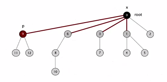
All we need is just change a few lines of our find method.
def find(index)
  return index if @ids[index] == index

  @ids[index] = @ids[@ids[index]]
  find(@ids[index])
end
Well, it is time to test it!
Tests
I found some data sets. One of them includes 11 union operations, and another one 900.
class Benchmarks
  def tiny
    test File.read('./tiny_UF.txt')
  end

  def medium
    test File.read('./medium_UF.txt')
  end

  private
  def test(str)
    data = str.split("\n")
    size, pairs = data.shift, data

    Benchmark.bm(20) do |bm|
      %w(QuickFind QuickUnion WeightedQuickUnion WeightedQuickUnionPC).each do |uf_class|
        bm.report(uf_class) do
          uf = Object.const_get(uf_class).new size.to_i
          union(uf, pairs)
        end
      end
    end
  end

  def union(uf, pairs)
    pairs.each do |pair|
      p, q = pair.split(' ')
      uf.union(p.to_i, q.to_i)
    end
  end
end
# tiny data set
user system total real
QuickFind
0.000000 0.000000 0.000000 (0.002838)
QuickUnion
0.000000 0.000000 0.000000 (0.000091)
WeightedQuickUnion
0.000000 0.000000 0.000000 (0.000078)
WeightedQuickUnionPC
0.000000 0.000000 0.000000 (0.000056)
# medium data set
user system total real
QuickFind
0.060000 0.010000 0.070000 (0.051383)
QuickUnion
0.010000 0.000000 0.010000 (0.002796)
WeightedQuickUnion
0.000000 0.000000 0.000000 (0.001658)
WeightedQuickUnionPC
0.010000 0.000000 0.010000 (0.001589)As you can see, everything works as we expected and Weighted Quick-Union With Path Compression is the quickest algorithm.
Here's the Union-Find algorithms performance comparison:
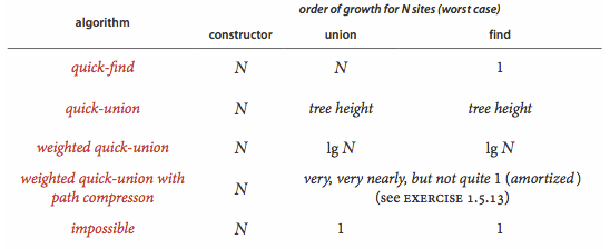
Union-Find algorithms performance comparisonConclusion
Union-Find algorithms are widely used. We can see them in different applications:
- Dynamic connectivity
- Games (Go)
- Percolation
- Least common ancestor
- Equivalence of finite state automata
- etc..
Thanks, Coursera for the amazing course and thank you for reading it 😛.
PS. More information about UF algorithms can be found in the course-related book's chapter.